Geiger Counter Experiment #2

Sources of Background Radiation

Everyone on the Earth is exposed to background radiation. Therefore, it is important to establish the sources of our background radiation. The three primary sources are; radiation from space (cosmic rays) and terrestrial (Earth) and internal (for our own body). Cosmic radiation from deep space and some released from our Sun during solar flares account for 8% of natural radiation exposure. Terrestrial radiation from rocks and soil accounts for 8% of natural radiation exposure. Added to the terrestrial radiation is radon. Radon, which is an invisible heavier than air gas emitted by uranium and thorium, accounts for about 65% of natural radiation exposure. Finally internal radiation, our bodies also contain radioactive materials, like potassium-40, which account for approximately 11% of natural radiation exposure.

Why Measure Background Radiation?

In order to make accurate measurements for some experiments you may need to subtract the background radiation from your measurements in order to obtain meaningful results.

For example, if you are measuring material that is emitting low levels of radioactivity you would need to subtract the background radiation to determine the radioactivity level of the material.

Going a little further, suppose you needed to check to see if a material is radioactive at all. Here not only do you need to know the background radiation, but the standard deviation which would help to determine if the radioactivity level you are reading is high or a normal fluctuation in the background radiation.

To take a measurement we first need to read our Geiger counter instrument.

How to set-up and read a Digital Geiger Counter

The GCA-07, GCA-06 and GCA-03 Series of digital Geiger counters have similar digital displays. The digital display has a number of advantages over analog meters, such as providing an exact count of the detected radioactive particles and their equivalent radiation level.

While the picture shows the front panel of the GCA-07W, the other series of Digital Geiger counters, GCA-06 and GCA-03 series all have similar controls.

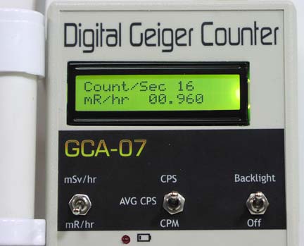
For instructions on using the GCA-07W please refer back to the Introduction To The GCA-07W.

Taking Background Radiation Measurements

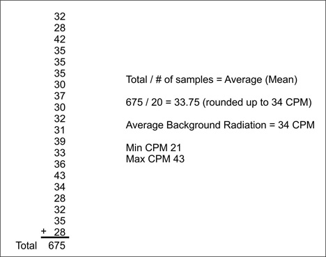
We use the CPM mode of the Geiger counter to take background radiation measurements. Position the Geiger counter or the Geiger counter’s sensor in an area that is free from external radioactive sources. Take a minimum of 10 CPM measurements and log the CPM number in a notebook. In the example shown below, 20 CPM measurements were recorded then added together for a total. Divide the total by the number of samples, in this case 20. This will be your average CPM or background radiation. In addition, note the highest and lowest CPM numbers you obtain in your sample. This will be you Max and Min.

Mean (Average)

In general, the higher the number of samples you record the greater the accuracy.

You can use this basic background radiation number to check objects in your environment for radioactivity. Place the wand of the Geiger counter on or near the suspect object and take a few CPM readings. For instance, I placed the wand on the screen of a working old style B/W television. This type of television uses a cathode ray tube to create a picture. My CPM reading was 65. Using the information above, you could conclude that the Cathode ray tube may be emitting soft x-rays.

The time scale shown below is in CPM and shows the background radiation for sixty CPM reading.

To finish this section take 10 or 20 CPM readings from your Geiger counter. Keep the Geiger counter or sensor away from any external source of radioactivity. Total the CPM readings and divide by the number of samples to obtain your average background CPM.

Part 2. Statistical Analysis of Background Radiation

In addition to calculating the average background radiation is calculating the sample standard deviation. The standard deviation quantifies the variance in the CPM readings. The standard deviation determines how far a CPM reading is from the mean (average). This can be useful when performing experiments where one may be trying to determine where a particular CPM reading falls, whether it is reasonably inside the sample group or outside the sample group.

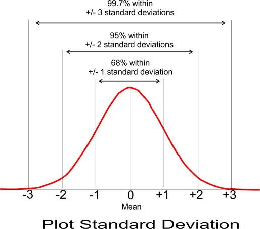
The chart below illustrates the general standard deviation. From the graph, 68% of values are found within 1 standard deviation from the mean. 95% of values are found within 2 standard deviations from the mean. Finally, 99.7% of values are found within 3 standard deviations from the mean.

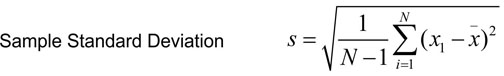
The formula for the sample standard deviation follows. The symbol s is the sample standard deviation. The summation sign iterates each CPM value 1 through 20 through the formula and sums them together. The variable x₁ are the CPM values. The symbol is the sample mean (average). The results of ( x1 - ‾x ) are squared ( x1 - ‾x )² then added to sum. When all CPM numbers have go through the formula, and are summed together, that result is multiplied by 1/20-1 or 1/19. Taking the square root of that result is the standard deviation.

How to Calculate Mean and Standard Deviation Manually:

Step 1) Determine mean of the CPM test results.
Step 2) Calculate difference between mean and individual test results.
Step 3) Calculate the square of individual results from Step 2
Step 4) Determine the sum of the values that were calculated in step 3.
Step 5) Calculate the standard deviation by dividing the sum from Step 4 by the number of tests minus 1, and then get the square root of that number.

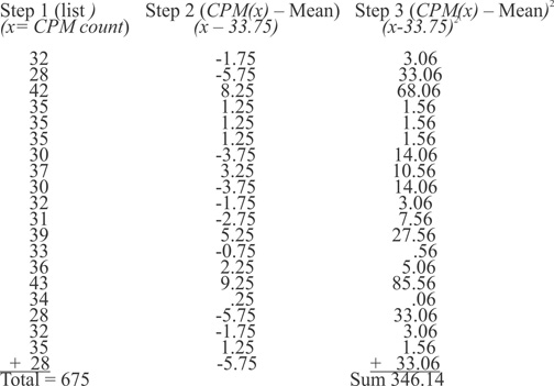
(Average) Mean = 675 / 20 = 33.75

(Step 1) To get the average, divide the Total by the number of samples. (Step 2) Then subtract the calculated average from each sample. (Step 3) Square the results of Step 2. (Step 4) Sum all results in step 3. (Step 5) Use the sum result to calculate the sample standard deviation using the following equation:

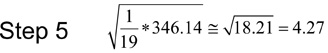
The standard deviation for these 20 CPM samples is 4.27. So for this group the mean is 33.75 and the standard deviation is 4.27

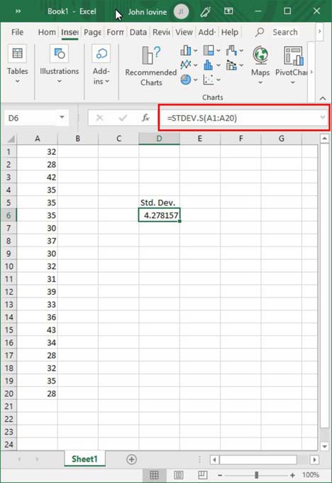
Using Excel to calculate Mean and Standard Deviation

Obtain 10 0r 20 sample CPM readings from your Geiger counter. If you are using Images Geiger Graphing software, you can save CPM data to a file that can be directly imported into Excel. If not you can enter the data manually.

Put the CPM values in the A column. In the screen below, the column A1 to A20 is filled with the 20 CPM values from our sample. Choose a cell to display the Standard Deviation result. In the figure below I choose cell D6. In the formula field above, see red box, enter the following formula =STDEV.S(A1:A20) and hit return. The cell will display the standard deviation. The Standard Deviation matches our manual calculation.

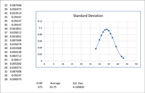
Going Further with Excel

You can do more with Excel than what is shown. For instance, Excel is also capable of plotting the standard deviation of the data points collected.

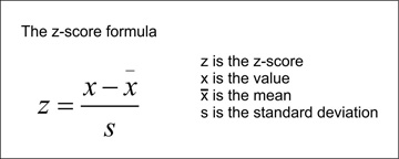
Z-Score

The z-score is the calculation of how many standard deviations a number is from the mean. For example, suppose we obtained a reading of 27 CPM. The value of 27 CPM would have a z-score of 1.61, since the value if 27 is 1.61 standard deviations from the mean.

To convert a value to its z-score do the following:

Subtract the value from the mean 33.75 - 27=6.75
Divide that result by the standard deviation 6.75 / 4.17 = 1.61

Practical Application - Example 1

In the case where we were checking an unknown material to see if it were radioactive. Assume we were reading CPM counts in the 50 to 60 CPM range. We know our mean is 33.75 CPM, rounded off to 34 CPM. Our standard deviation is 4.27. The counts we are reading are more than 3 standard deviations from our mean. We could say with a high degree of confidence that the material is radioactive.

Practical Application - Example 2

In the case where we were checking a second unknown material to see if it were radioactive. Assume we were reading CPM counts in the 40 CPM range. We know our mean is 33.75 CPM, rounded off to 34 CPM. Our standard deviation is 4.27. The counts we are reading are within 2 standard deviations from our mean. We could reasonable conclude that the 40 CPM reading could be a normal fluctuation in our background radiation.

Practical Application - Example 3

In the case where I checked for radiation being emitted from an old cathode ray TV tube and obtained a CPM reading of 65 CPM. This reading falls outside 3 standard deviations from the mean. We could reasonably conclude that the cathode ray tube is emitting soft x-rays.

Online Calculators for Performing Math

Euler's Number = 2.718281